- It’s time to apply Classification Model into practice!
- The notes would cover: Data Description, Logistic Regression, LDA, QDA, KNN and an Example
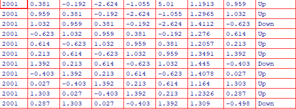
Stock Market Data
- percentage returns for the S&P 500 stock index over 1250 days, from 2011 to end of 2005.
- Load the data
1 | library(ISLR) |
- A glance at the dataset:

- Use
cor(matrix)to view the correlations between predictors, if some predictors are qualitative, they should be removed
1 | cor(Smarket[,-9]) |
Logistic Regression
Model
- Use
glm(model formula)to fit a generalized linear model including logistic regression, indicated by pass family=binomial
1 | glm.fit = glm(Direction~Lag1+Lag2+Lag3+Lag4+Lag5+Volume,data=Smarket,family=binomial) |
- Refit the model using subset of data:
1 | glm.fit = glm(Direction~Lag1+Lag2+Lag3+Lag4+Lag5+Volume,data=Smarket,family=binomial,subset=train) |
- Refit the model using less predictors:
1 | glm.fit = glm(Direction~Lag1+Lag2, data=Smarket,family=binomial,subset=train) |
Predict
predict(glm.fit)predict the logit($\beta_0+\beta_1X$)predict(glm.fit,type=response)predict the probability of up- The value is the probability of up because of what
contrasts(Direction)show
1 | > contrasts(Direction) |
- Convert the predict value to label
1 | glm.pred = rep("Down",1250) |
- To predict a particular day
1 | predict(glm.fit,newdata=data.frame(Lag1=c(1.2,1.5),Lag2=c(1.1,-0.8)),type="response") |
Assessment
Confusion Matrix
1 | table(glm.pred,Direction) |
Correction Rate
1 | mean(glm.pred==Direction) |
Separate the training data
1 | train = (Year<2005) |
- The same code in Python would be:
Smarket['2005'] = Smarket[Smarket.Year>2005]Direction['2005'] = Smarket[Smarket.Year>2005].Direction
Refit
- See the above
Re-assess(subset data)
1 | glm.pred = rep("Down",252) |
Re-assess(less predictor)
1 | glm.pred = rep("Down",252) |
LDA
Fit Model
- Use
lad(formula)to fit a LDA model, which is part ofMASSpackage
1 | lda.fit = lda(Direction~Lag1+Lag2,data=Smarket,subset=train) |
- result:
1 | Call: |
Assessment
plot(lda.fit)produces plot of the linear discriminantslda.pred=predict(lda.fit,Smarket.2005)names(lda.pred)- class contains LDA’s predictions about the movement of the market
- posterior a matrix whose kth column contains the posterior probability belong to the kth class
- x contains the linear discriminants
lda.class = lda.pred$classtable(lda.class,Direction.2005)mean(lda.class==Direction.2005)
Change the Threshold
sum(lda.pred$posterior[,1]>=0.5)sum(lda.pred$posterior[,1]>0.9)* remember to test whether class is correspond to the larger probability
lda.pred$posterior[1:20,1]lda.class[1:20]
KNN
Data Cleaning
1 | train.X = cbind(Lag1,Lag2)[train,] |
The knn() Method
- A part of
classpackage knn()require four inputs:- matrix containing the predictors associated with the training data
- matrix containing the test dataset
- vector containing the class labels for training observations
- value for K, the level of flexibility
1 | library(class) |
Application to Caravan Insurance Data
Data set
- Caravan data set, a part of ISLR library
- Includes 85 predictors that measure demographic characteristics for 5822 individuals, of which 348 purchase the insurance.

- Important: The scale of the predictor matter a lot to KNN, so we should standardize the dataset before we apply the method. 也就是说,如果某个维度上scale比较大,那么这个点就会相当远
Data Cleaning
- Standardization
1 | standardized.X = scale(Caravan(,-86)) |
- Split the dataset
1 | test = 1:1000 |
Model Fitting
1 | set.seed(1) |
Discussion
The error rate is 12. However, if we just predict every customer would not purchase, the error rate is 6%.
But, if the company wants to sell insurance to those who want to but it, it’s worth noting that:
- The rate of TP/P* is 0.117, which means among 77 who were predicted to be true, 9 are right-predicted.
However, the random guess is 6%
Change the K to 5 yields:
1 | knn.pred = knn(train.X,test.X,train.Y,k=5) |
- When we apply logistic regression:
1 | glm.fit = glm(Purchase~.,data = Caravan,family=binomial,subset=-test) |